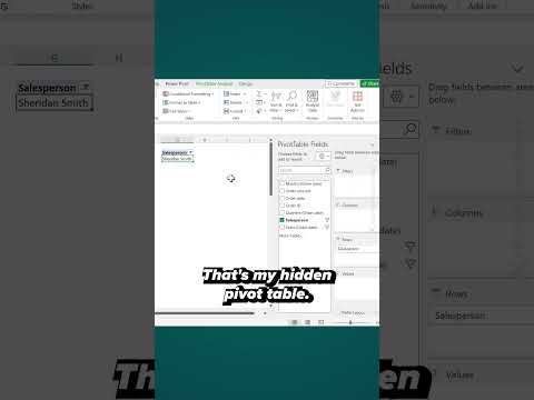
Cool Excel Trick Use Slicer Buttons With a Hidden Pivot Table
Here is a simple Excel trick on how to use Pivot Table slicers in a formula based report.
Cool Excel Trick Use Slicer Buttons With a Hidden Pivot Table. This Excel trick teaches how to use Pivot Table slicers in a formula-based report. You can connect your formulas to slicer buttons using a hidden Microsoft Excel Pivot Table and link the pivot table outcome to the Excel formulas.
Here are the steps on how you can set it up:
- Start with your data, for example, a table with sales data.
- Insert a PivotTable based on this data.
- Adjust your PivotTable as needed, for example, sales by region or by month.
- With the PivotTable selected.
- Click on the "Insert Slicer" button.
- Choose the field you want the slicer for, such as Region or Month.
- Suppose you also have a chart that is based on some of the same data, but not directly on the PivotTable.
- You can connect the slicer to that chart to allow it to control the chart.
- Select the slicer.
- Click on "Report Connections".
- Check the boxes for any other PivotTables or PivotCharts you want this slicer to control.
- After setting up your slicer and connected it to the relevant tables or charts, you might need to hide the original PivotTable.
- Click on the sheet tab where the PivotTable is located.
- Right-click and choose "Hide". Alternatively, you can simply move the PivotTable to a new sheet and not display that sheet to the end-users.
- Select the slicer.
- Use the available options to style the slicer according to your preference.
- You can alter the color, the number of columns, button styles, etc.
- Create a PivotTable:
- Insert a Slicer:
- Connect the Slicer to another Table/Chart:
- Hide the PivotTable:
- Style the Slicer (Optional):
This trick allows you to have a slicer controlling a chart or table without the original PivotTable being visible. This can make your Excel reports or dashboards look tidier and more professional.
Main Topic: Excel Slicer Buttons With Hidden PivotTable
The main topic of this trick is using Excel slicer buttons with a hidden PivotTable. This adds more versatility and makes report or dashboard operation simpler. PivotTable slicers in Excel provide a quick way to filter data interactively, which can be very useful for data analysis and report generation. By hiding the original PivotTable and allowing the slicer to control a table or chart, you make the report less cluttered and more straightforward for users, improving your report's overall quality and user experience.
Learn about Cool Excel Trick Use Slicer Buttons With a Hidden Pivot Table

The main topic of the text is about using slicer buttons with a hidden pivot table in Microsoft Excel for a more interactive, user-friendly report or dashboard. The text provides a guide on how to create a pivot table from sales data, insert a slicer, and then connect the slicer to another chart or table. After setting up and connecting the slicer, the original pivot table can be hidden for a cleaner and more professional presentation. Slicers provide interactive functionality without the need for the original pivot table to be visible. Notably, the slicer can also be styled to fit user preferences.
More links on about Cool Excel Trick Use Slicer Buttons With a Hidden Pivot Table
- Excel Slicer Trick
- Oct 13, 2015 — In this Excel Slicer Trick I show you how to use a Slicer to display a drilled down view of your data in a PivotChart.
- 101 Advanced Pivot Table Tips And Tricks You Need To ...
- This collection of awesome tips and tricks will help you master pivot tables and become a data ninja! You're gonna learn all the tips the pros use, ...
- The Ultimate Guide to Excel Pivot Table Slicers
- Apr 1, 2021 — Excel Slicers are visual filters/interactive buttons that allow you to see what Pivot Table items have been selected. Click here to learn ...
- Using Slicers in Excel Pivot Table - A Beginner's Guide
- In this tutorial, you'll learn how to insert and use slicers in Excel. It also covers slicers formatting and other useful features.
- 6 Advanced Pivot Table Techniques
- 1. Use slicers · 2. Create a calculated field · 3. Create multiple pivot tables from one · 4. Hide or unhide subtotals · 5. Look behind the scenes of your pivot ...
- How to Include Measures (or KPIs) inside Slicers - Excel ...
- Sep 9, 2021 — How to Include Measures (or KPIs) inside Slicers – Excel Interactive Dashboard Trick · Step 1: Create a Pivot Table Using the Data Model · Step 2: ...
Keywords
Microsoft Excel Slicer Trick, Hidden PivotTable with Slicer in Excel, Excel PivotTable Slicer without Displaying, Interactive Excel Dashboard with Slicer, Advanced Excel Slicer Usage.